Project Name: Chaos Theory and The Game of Chaos
I. Theory
1. Introduction
Chaos theory is a study that concerns the predictablity of a system. For example, the position of a simple pendulum can be predicted very accurately, while the end positions of a system that consists of two interconnected pendulums are hard to predict.
(image adapted from: http://community.wolfram.com//c/portal/getImageAttachment?filename=tumblr_n5r8wbYqFr1tzs5dao1_1280.gif&userId=11733)
By definition, chaotic systems are system that can be described as a system of interconnected differential equations (usually impossible to solve, but they have some special case solutions).
2. Examples - Three Body System
Consiter a 3-Body system:
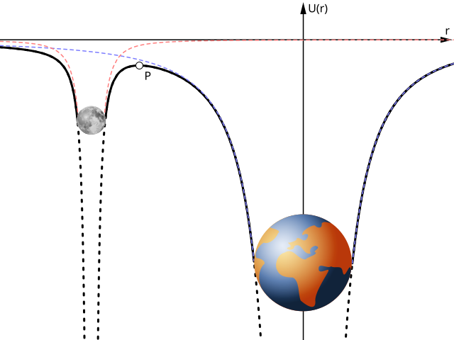
(image adapted from: https://upload.wikimedia.org/wikipedia/commons/thumb/8/86/Earth-moon-gravitational-potential.svg/640px-Earth-moon-gravitational-potential.svg.png)
The force of one planet, planet C, can be calculated by combining two other gravitational potential of the bodies (planet A, planet B). And therefore, if those two gravitational potential (planet A, planet B) stay the same, we can 100% predict where the planet C is going to end up.
However, the two other gravitational potential (planet A, planet B) is affected by the planet C, it becomes a chaotic system.
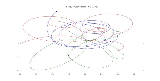
(image adapted from: https://www.epsilontheory.com/wp-content/uploads/epsilon-theory-the-three-body-problem-december-21-2017-graph-one.jpg)
3. Characteristics of Chaotic System
There are some characteristics of a chaotic system we
II. Experiment
The following experiments are my investigation on the characteristics of chaotic systems that helped me to build my project - The Game of Chaos.
0x00 Write N-Body Simulation Program
# -*- coding: utf-8 -*-
"""
N-body problem simulation for matplotlab. Based on
https://fiftyexamples.readthedocs.org/en/latest/gravity.html
Credit: https://github.com/brandones/n-body
"""
import argparse
import random
import itertools
import json
from math import atan2, sin, cos
from time import sleep

import numpy as np
import math

import matplotlib.animation as animation
from mpl_toolkits.mplot3d import Axes3D
import matplotlib.pyplot as plt
from matplotlib.widgets import Slider, Button


# Constants and Configurations
G = 6.67428e-11
AU = (149.6e6 * 1000)
ONE_DAY = 24*3600
TRACK_NUM = 1

# Serialization Utility
class BodyEncoder(json.JSONEncoder):
    def default(self, obj):
        if isinstance(obj, np.ndarray):
            return obj.tolist()
        if hasattr(obj, '__jsonencode__'):
            return obj.__jsonencode__()
        if isinstance(obj, set):
            return list(obj)
        return obj.__dict__

    def deserialize(data):
        bodies = [Body(d["name"],d["mass"],np.array(d["p"]),np.array(d["v"])) for d in data["bodies"]]
        axis_range = data["axis_range"]
        timescale = data["timescale"]
        return bodies, axis_range, timescale

    def serialize(data):
        file = open('data.json', 'w+')
        json.dump(data, file, cls=BodyEncoder, indent=4)
        return json.dumps(data, cls=BodyEncoder, indent=4)

# Body Object
class Body(object):
    def __init__(self, name, mass, p, v=(0.0, 0.0, 0.0)):
        self.name = name
        self.mass = mass
        self.p = p
        self.v = v
        self.f = np.array([0.0, 0.0, 0.0])

    def __str__(self):
        return 'Body {}'.format(self.name)

    def attraction(self, other):
        """Calculate the force vector between the two bodies"""
        assert self is not other
        diff_vector = other.p - self.p
        distance = norm(diff_vector)

        # Remove Collision
        # assert np.abs(distance) < 10**4, 'Bodies collided!'

        # F = GMm/r^2
        f_tot = G * self.mass * other.mass / (distance**2)
        # Get force with a direction
        f = f_tot * diff_vector / distance
        return f

    # def __dict__(self):
    #     return {"name": self.name, "mass": self.mass, "p": self.p.tolist(), "v": self.v.tolist(), "f": self.f.tolist()}


def norm(x):
    """return: vector length in n demension"""
    return np.sqrt(np.sum(x**2))


def move(bodies, timestep):
    # combinations('ABCD', 2) --> AB AC AD BC BD CD
    # combinations(range(4), 3) --> 012 013 023 123
    pairs = itertools.combinations(bodies, 2)

    # Initialize force vectors
    for b in bodies:
        b.f = np.array([0.0, 0.0, 0.0])

    # Calculate force vectors
    for b1, b2 in pairs:
        f = b1.attraction(b2)
        b1.f += f
        b2.f -= f

    # Update velocities based on force, update positions based on velocity
    # Approximate as linear acceleration
    for body in bodies:
        # v = at = (F/m)t
        body.v += body.f / body.mass * timestep
        # x = vt
        body.p += body.v * timestep

def points_for_bodies(bodies):
    x0 = np.array([body.p[0] for body in bodies])
    y0 = np.array([body.p[1] for body in bodies])
    z0 = np.array([body.p[2] for body in bodies])
    return x0, y0, z0

def norm_forces_for_bodies(bodies, norm_factor):
    u0 = np.array([body.f[0] for body in bodies])
    v0 = np.array([body.f[1] for body in bodies])
    w0 = np.array([body.f[2] for body in bodies])
    return u0/norm_factor, v0/norm_factor, w0/norm_factor


class AnimatedScatter(object):
    def __init__(self, bodies, axis_range, timescale, stop_time, interval=1):
        self.n_frame = 0
        self.stop_time = stop_time
        self.interval = interval

        self.bodies = bodies
        self.axis_range = axis_range
        self.timescale = timescale
        self.stream = self.data_stream()

        self.force_norm_factor = None
        if self.interval != 0:
            fig = plt.figure()
            ax = fig.add_subplot(111, projection='3d')
            self.fig = fig
            self.ax = ax
            self.ani = animation.FuncAnimation(self.fig, self.update, interval=self.interval,
                                               init_func=self.setup_plot, blit=False)

        self.x_ = []
        self.y_ = []
        self.z_ = []
        self.last_yield = None


    def setup_plot(self):
        xi, yi, zi, ui, vi, wi, x_, y_, z_ = next(self.stream)

        c = [np.random.rand(3,) for i in range(len(xi))]

        self.ax.set_proj_type('ortho')
        self.scatter = self.ax.scatter(xi, yi, zi, c=c, s=10)
        self.quiver = self.ax.quiver(xi, yi, zi, ui, vi, wi, length=1)
        self.lines, = self.ax.plot([], [], [], ".", markersize=0.5)

        self.axtime = plt.axes([0.25, 0.1, 0.65, 0.03])
        self.stime = Slider(self.axtime, 'Time', 0.0, 10.0, valinit=0.0)
        def update(val):
            if val == 0: return
            print("Jumping e^{}={} frames".format(int(val), int(math.e**val)))
            for v in range(int(math.e**val)):
                x_i, y_i, z_i, u_i, v_i, w_i, x_, y_, z_  = next(self.stream)
            self.stime.reset()
        self.stime.on_changed(update)

        self.resetax = plt.axes([0.8, 0.025, 0.1, 0.04])
        self.button = Button(self.resetax, 'Reset', hovercolor='0.975')
        def reset(event):
            self.stime.reset()
            self.x_ = []
            self.y_ = []
            self.z_ = []
        self.button.on_clicked(reset)

        FLOOR = self.axis_range[0]
        CEILING = self.axis_range[1]
        self.ax.set_xlim3d(FLOOR, CEILING)
        self.ax.set_ylim3d(FLOOR, CEILING)
        self.ax.set_zlim3d(FLOOR, CEILING)
        self.ax.set_xlabel('X')
        self.ax.set_ylabel('Y')
        self.ax.set_zlabel('Z')

        return self.scatter, self.quiver

    def quiver_force_norm_factor(self):
        axis_length = np.abs(self.axis_range[1]) + np.abs(self.axis_range[0])
        return np.amax(np.array([b.f for b in self.bodies]))/(axis_length/10)

    def data_stream(self):
        while self.n_frame < self.stop_time:
            self.n_frame = self.n_frame + 1
            move(self.bodies, self.timescale)
            if not self.force_norm_factor:
                self.force_norm_factor = self.quiver_force_norm_factor()
                # print('factor ', self.force_norm_factor)
            x, y, z = points_for_bodies(self.bodies)
            u, v, w = norm_forces_for_bodies(self.bodies, self.force_norm_factor)

            # rad = random.randint(0, TRACK_NUM-1)
            # x_.append(x[rad])
            # y_.append(y[rad])
            # z_.append(z[rad])

            self.x_.append(x[-1])
            self.y_.append(y[-1])
            self.z_.append(z[-1])
            yield x, y, z, u, v, w, self.x_, self.y_, self.z_

    def update(self, i):
        x_i, y_i, z_i, u_i, v_i, w_i, x_, y_, z_  = next(self.stream)
        self.last_yield = (x_i, y_i, z_i, u_i, v_i, w_i, x_, y_, z_)

        self.scatter._offsets3d = (x_i, y_i, z_i)

        segments = np.array([(b.p, b.p + b.f/self.force_norm_factor) for b in self.bodies])
        self.quiver.set_segments(segments)

        self.lines.set_data(np.array(x_), np.array(y_))
        self.lines.set_3d_properties(np.array(z_))

        plt.draw()
        return self.scatter, self.quiver, self.lines

    def show(self):
        if self.interval != 0:
            plt.show()
        else:
            while self.n_frame < self.stop_time:
                self.n_frame = self.n_frame + 1
                self.last_yield = next(self.stream)
            return self

def parameters_for_simulation(simulation_name, file_name=None):

    if simulation_name == 'solar':
        sun = Body('sun', mass=1.98892 * 10**30, p=np.array([0.0, 0.0, 0.0]))
        earth = Body('earth', mass=5.9742 * 10**24, p=np.array([-1*AU, 0.0, 0.0]), v=np.array([0.0, 29.783 * 1000, 0.0]))
        venus = Body('venus', mass=4.8685 * 10**24, p=np.array([0.723 * AU, 0.0, 0.0]), v=np.array([0.0, -35.0 * 1000, 0.0]))
        axis_range = (-1.2*AU, 1.2*AU)
        timescale = ONE_DAY
        return (sun, earth, venus), axis_range, timescale

    elif simulation_name == 'dump':
        data = json.loads(open(file_name, "r").read())
        return BodyEncoder.deserialize(data)

    elif simulation_name == 'random_three':
        n = 2
        position = AU/150
        time = 100.
        speed = 0.2
        bodies = []
        for i in range(n):
            name = 'random_{}'.format(n)
            mass = random.uniform(4.0**24,6.0**24)
            p = np.array([random.uniform(-position, position), random.uniform(-position, position), random.uniform(-position, position)])
            v = np.array([random.uniform(-speed, speed),random.uniform(-speed, speed),random.uniform(-speed, speed)])
            # v = np.array([0.,0.,0.])
            bodies.append(Body(name, mass=mass, p=p, v=v))
            # print("Appending {}, {}, {}, {}".format(name, mass, p, v))
        bodies.append(Body("sun", mass=5.0**24, p=np.array([0.,0.,0.])))

        axis_range = (-2*position, 2*position)
        timescale = ONE_DAY*time
        return tuple(bodies), axis_range, timescale

    elif simulation_name == 'random':
        n = 49
        position = AU/150
        time = 100.
        speed = 2.
        bodies = []
        for i in range(n):
            name = 'random_{}'.format(n)
            mass = random.uniform(4.0**24,6.0**24)
            p = np.array([random.uniform(-position, position), random.uniform(-position, position), random.uniform(-position, position)])
            v = np.array([random.uniform(-speed, speed),random.uniform(-speed, speed),random.uniform(-speed, speed)])
            # v = np.array([0.,0.,0.])
            bodies.append(Body(name, mass=mass, p=p, v=v))
            # print("Appending {}, {}, {}, {}".format(name, mass, p, v))
        bodies.append(Body("sun", mass=6.5**24, p=np.array([0.,0.,0.])))

        axis_range = (-2*position, 2*position)
        timescale = ONE_DAY*time
        return tuple(bodies), axis_range, timescale

    elif simulation_name == 'negative_random':
        n = 20
        position = AU
        time = 10.
        speed = 1000.
        bodies = []
        for i in range(n):
            name = 'random_{}'.format(n)
            mass = random.uniform(-1.0**23,-2.0**24)
            p = np.array([random.uniform(-position, position), random.uniform(-position, position), random.uniform(-position, position)])
            v = np.array([random.uniform(-speed, speed),random.uniform(-speed, speed),random.uniform(-speed, speed)])
            # v = np.array([0.,0.,0.])
            bodies.append(Body(name, mass=mass, p=p, v=v))
            # print("Appending {}, {}, {}, {}".format(name, mass, p, v))
        bodies.append(Body("sun", mass=-9.0**24, p=np.array([0.,0.,0.])))

        axis_range = (-2*AU, 2*AU)
        timescale = ONE_DAY*time
        return tuple(bodies), axis_range, timescale

    elif simulation_name == 'mix_random':
        n = 20
        position = AU
        time = 10.
        speed = 1000.
        bodies = []
        for i in range(n):
            name = 'random_{}'.format(n)
            mass = random.choice([random.uniform(-1.0**21,-2.0**20), random.uniform(1.0**23,2.0**24), random.uniform(1.0**23,2.0**24), random.uniform(1.0**23,2.0**24)])
            p = np.array([random.uniform(-position, position), random.uniform(-position, position), random.uniform(-position, position)])
            v = np.array([random.uniform(-speed, speed),random.uniform(-speed, speed),random.uniform(-speed, speed)])
            # v = np.array([0.,0.,0.])
            bodies.append(Body(name, mass=mass, p=p, v=v))
            # print("Appending {}, {}, {}, {}".format(name, mass, p, v))
        bodies.append(Body("sun", mass=-9.0**24, p=np.array([0.,0.,0.])))

        axis_range = (-2*AU, 2*AU)
        timescale = ONE_DAY*time
        return tuple(bodies), axis_range, timescale

    elif simulation_name == 'misc3':
        """
        This is basically mostly just a demonstration that this
        simulation doesn't respect conservation laws.
        """
        sun1 = Body('A', mass=6.0 * 10**30, p=np.array([4.0*AU, 0.5*AU, 0.0]), v=np.array([-10.0 * 1000, -1.0 * 1000, 0.0]))
        sun2 = Body('B', mass=8.0 * 10**30, p=np.array([-6.0*AU, 0.0, 3.0*AU]), v=np.array([5.0 * 1000, 0.0, 0.0]))
        sun3 = Body('C', mass=10.0 * 10**30, p=np.array([0.723 * AU, -5.0 * AU, -1.0*AU]), v=np.array([-10.0 * 1000, 0.0, 0.0]))
        axis_range = (-20*AU, 20*AU)
        timescale = ONE_DAY
        return (sun1, sun2, sun3), axis_range, timescale

    elif simulation_name == 'centauri3':
        """
        Based on known orbit dimensions and masses.
        Not working, not sure why. They shouldn't get farther than 36AU
        or about 5e12m away from each other.
        """
        p_a = np.array([-7.5711 * 10**11, 0.0, 0.0])
        p_b = np.array([9.1838 * 10**11, 0.0, 0.0])
        v_a = np.array([0.0, 1.212 * 10**4, 0.0])
        v_b = np.array([0.0, -1.100 * 10**4, 0.0])
        alphaA = Body('Alpha A', mass=1.100*1.98892 * 10**30, p=p_a, v=v_a)
        alphaB = Body('Alpha B', mass=0.907*1.98892 * 10**30, p=p_b, v=v_b)
        axis_range = (-10.0**13, 10.0**13)
        timescale = ONE_DAY * 5
        return (alphaA, alphaB), axis_range, timescale

    else:
        raise ValueError('No simulation named {}'.format(simulation_name))
0x02 Run a Simulation
Generate a random configuration:
%matplotlib notebook
MODE = "random"
DATA_LEN = 10000

bodies, axis_range, timescale = parameters_for_simulation(MODE)
data = {"bodies": bodies, "axis_range": axis_range, "timescale": timescale}

a = AnimatedScatter(bodies, axis_range, timescale, DATA_LEN, 1)
a.show()

Here, I used generated random 3-body configuration to run a simple simulation. Everything, including position, mass, initial velocity of the planets/suns are randomly chosen. The tregectory of one planet/sun is graphed in 3D space shown below.
%matplotlib notebook
FILE_NAME = "random_three_twisted.json"
MODE = "dump"
DATA_LEN = 10000
# DATA_LEN = 10800

bodies, axis_range, timescale = parameters_for_simulation(MODE, file_name=FILE_NAME)
data = {"bodies": bodies, "axis_range": axis_range, "timescale": timescale}
print(BodyEncoder.serialize(data))

a = AnimatedScatter(bodies, axis_range, timescale, DATA_LEN, 1)
a.show()

0x03 Get the End Points of the Simulation
Because we want to twick the initial setting by a little bit, in this case, the initial velocity of one planet, to see how the end position change, we need to first write a function that gives the end position of the planet.
x_i, y_i, z_i, u_i, v_i, w_i, x_, y_, z_ = a.last_yield
points = []
for i in zip(x_, y_, z_):
    points.append(i)

points = np.array(points)
print(points)
print("len(points) = {}".format(len(points)))
def get_last_point(time=10000, data=None):
    if data is None:
        FILE_NAME= "random_three_twisted.json"
        MODE = "dump"
        DATA_LEN = time

        bodies, axis_range, timescale = parameters_for_simulation(MODE, file_name=FILE_NAME)
    else:
        bodies, axis_range, timescale = data

    a = AnimatedScatter(bodies, axis_range, timescale, time, interval=0)
    a.show()

    x_i, y_i, z_i, u_i, v_i, w_i, x_, y_, z_ = a.last_yield
    return x_[-1], y_[-1], z_[-1]
print("The last point of the simulation after some time t is {}".format(get_last_point(time=10000, data=None)))
0x04 Plot a simple Bifurcation Logistic Map
In this section, we twick the initial velocity in x direction of planet 2 from 0 m/s to 0.0058 m/s by 1000 steps. Then, I graphed its 3D position in the 3D space, the color indicates the initial velocity. Afterthat, I graphed distance between the body and its initial position as a function of initial velocity.
from tqdm import tqdm_notebook as tqdm

def get_bifurcation(linspace=None):
    l = []
    pbar = tqdm(linspace)
    for i in pbar:
        FILE_NAME= "random_three_twisted.json"
        MODE = "dump"

        bodies, axis_range, timescale = parameters_for_simulation(MODE, file_name=FILE_NAME)
        bodies[1].v = np.array([i, 0.04193708594602602, 0.023326091537453186])
        point = get_last_point(time=10000, data=(bodies, axis_range, timescale))
        pbar.set_description("bodies[1].v = {}, point = {}".format(bodies[1].v, point))
        l.append(point)
    return np.array(l)
result = None
try:
    result = np.load("0.npy")
except FileNotFoundError as e:
    linspace = np.linspace(0, 0.0058, 1000)
    result = get_bifurcation(linspace)
    np.save("0.npy", result)

print(result)
In the cell below, we can see that a large amount of the points are in the center of the graph, while some scatter around the 3D space randomly.
fig = plt.figure()
ax = plt.axes(projection='3d')

fig.suptitle('End Points of a Planet After 1,000,000 Days', fontsize=14, fontweight='bold')
ax.set_title('The color of the dot represent different \n initial velocity of the planet from v=0m/s to v=0.0058m/s \n')
ax.set_xlabel('X (m)')
ax.set_ylabel('Y (m)')
ax.set_zlabel('Z (m)')

ax.scatter3D(result[:,0], result[:,1], result[:,2], c=range(len(result)), cmap='plasma');
fig.show()

In the cell below, we can see the position is resilient when the initial velocity is between #20 to #80 steps, while they are truely random between #0 and #20
vector_len = np.array([norm(i) for i in result])
# print(vector_len)
fig = plt.figure()
x = np.linspace(0, 0.0058, 1000)
y = vector_len
plt.scatter(x, y, c=vector_len, alpha=.9, s=8)
plt.plot(x, y, alpha=0.5)
plt.xlim(0, 0.0058)

ax = fig.add_subplot(111)
fig.suptitle('Distance to Origin of a Planet After 1,000,000 Days', fontsize=14, fontweight='bold')
ax.set_xlabel('Initial Velocity (m/s)')
ax.set_ylabel('Distance (m)')

fig.show()

def graph_3d_bifurcation(result, linspace):
    fig = plt.figure()
    ax = plt.axes(projection='3d')
    ax.scatter3D(result[:,0], result[:,1], result[:,2], c=linspace, cmap='plasma', alpha=.5, s=0.5);

    fig.suptitle('End Points of a Planet After 1,000,000 Days', fontsize=12, fontweight='bold')
    ax.set_title('The color of the dot represent different \n initial velocity of the planet from v={}m/s to v={}/s \n'.format(linspace[0], linspace[-1]))
    ax.set_xlabel('X (m)')
    ax.set_ylabel('Y (m)')
    ax.set_zlabel('Z (m)')

    fig.show()
def graph_2d_bifurcation(result, linspace, standard_resize=True):
    vector_len = np.array([norm(i) for i in result])
    fig = plt.figure()
    x = linspace
    y = vector_len
    plt.scatter(x, y, c=vector_len, alpha=.5, s=0.5)

    ax = fig.add_subplot(111)
    fig.suptitle('Distance to Origin of a Planet After 1,000,000 Days', fontsize=12, fontweight='bold')
    ax.set_title('Initial velocity from v={}m/s to v={}/s \n'.format(linspace[0], linspace[-1]))
    ax.set_xlabel('Initial Velocity (m/s)')
    ax.set_ylabel('Distance (m)')

    plt.xlim(linspace[0], linspace[-1])
    if standard_resize: plt.ylim(0, 2.0e12)
    fig.show()

# Not used in the project
def graph_hist_bifurcation(result, standard_resize=True):
    vector_len = np.array([norm(i) for i in result])
    print("Your score is: -{}".format(np.std(vector_len)))
    fig = plt.figure()
    ax = fig.add_subplot(111)
    y = vector_len

    plt.hist(y, normed=False, bins=100)
    plt.ylabel('Frequency');
    if standard_resize: plt.xlim(0, 1.0e12)

    fig.suptitle('Distance to Origin of a Planet After 1,000,000 Days', fontsize=14, fontweight='bold')
    fig.show()
result = None
try:
    result = np.load("1.npy")
except FileNotFoundError as e:
    linspace = np.linspace(0, 0.0058, 10000)
    result = get_bifurcation(linspace)
    np.save("1.npy", result)
graph_3d_bifurcation(np.load("1.npy"), np.linspace(0, 0.0058, 10000))

graph_2d_bifurcation(np.load("1.npy"), np.linspace(0, 0.0058, 10000))

Lets zoom in between 0.000 and 0.001
result = None
try:
    result = np.load("2.npy")
except FileNotFoundError as e:
    linspace = np.linspace(0, 0.0010, 10000)
    result = get_bifurcation(linspace)
    np.save("2.npy", result)
graph_3d_bifurcation(np.load("2.npy"), np.linspace(0, 0.0010, 10000))

graph_2d_bifurcation(np.load("2.npy"), np.linspace(0, 0.0010, 10000))

Lets zoom in again between 0.0006 and 0.0008
result = None
try:
    result = np.load("3.npy")
except FileNotFoundError as e:
    linspace = np.linspace(0.0006, 0.0008, 10000)
    result = get_bifurcation(linspace)
    np.save("3.npy", result)
graph_3d_bifurcation(np.load("3.npy"), np.linspace(0.0006, 0.0008, 10000))

graph_2d_bifurcation(np.load("3.npy"), np.linspace(0.0006, 0.0008, 10000))

Lets zoom in again between 0.00065 and 0.000675
result = None
try:
    result = np.load("4.npy")
except FileNotFoundError as e:
    linspace = np.linspace(0.00065, 0.000675, 10000)
    result = get_bifurcation(linspace)
    np.save("4.npy", result)
graph_3d_bifurcation(np.load("4.npy"), np.linspace(0.00065, 0.000675, 10000))

graph_2d_bifurcation(np.load("4.npy"), np.linspace(0.00065, 0.000675, 10000))

Lets see the zoomed in version of the first graph where the end position is resilient.
result = None
try:
    result = np.load("5.npy")
except FileNotFoundError as e:
    linspace = np.linspace(0.0035, 0.0040, 10000)
    result = get_bifurcation(linspace)
    np.save("5.npy", result)
graph_3d_bifurcation(np.load("5.npy"), np.linspace(0.0035, 0.0040, 10000))

graph_2d_bifurcation(np.load("5.npy"), np.linspace(0.0035, 0.0040, 10000))

graph_2d_bifurcation(np.load("5.npy"), np.linspace(0.0035, 0.0040, 10000), standard_resize=False)

0x05 Observation
From the graph, we can see the following characteristics:
1. As I tweak the initial velocity of the planet, the distance is fluctuating within one range, and seldom surpass that range.
2. However, the actual distance to the origin appears to be random and densely covered within some range.
3. As we zoom in, I observe a pattern in the randomness due to the density of the periodic orbits.
4. As we zoom in, I still observe randomness in some region of initial velocity but I can also see some continuous lines created by data points.
0x06 Conclusion
From the images above, I can clearly see the characteristics of the chaotic system in these three body simulation.
1. Repetition: The distance between the final position of the planet and the origin oscillates between 0 to 1e12 meter.
2. The density of periodic orbits / Fractal Structure: As I zoom in, although I can see more details in the range I selected, I can still see randomly plotted dense dots under or between the periodic trends.
3. Sensitivity to initial conditions: Since there are infinite details in the graph, it suggests that an infinitely small change may cause sudden fluctuation between the range of values (in this case, 0 to 1e12 meter). Specifically, a relatively small change to its initial velocity around 0.000664 can result in a sudden jump in the final position to origin from 0m to 1.75e12m.
4. Strange attractors: Unlike fixed-point attractors and limit cycles, the attractor in the 3D simulation move as the simulation runs. Because the trajectories around attractors do not converge to a fixed value and may result in a fractal structure, the center is a sign of a strange attractor.
III. The Game of Chaos
1. Game Rule
In this game, you need to use your knowledge to build a relatively stable system. Because the score is based on the stability of the last planet, players should cooperate to build a stable system as possible.
- Think about the definition of chaotic systems
- Think about the differential equation of gravitational potential
- Think about what approximation can be used in definition of chaotic systems to make it less chaotic
- Think about how mass affect the stability of n-body system
- Be able to understand the output graph of the grame to adjust your strategy
2. Instruction
- This game allows about 3-10 players. Please enter the number of players below
NUMBER_OF_PLAYER = 4
- Please run the cell below and then plug the location and the velocity on the canvas created below the code. The program will generate a random mass of the planet for each player below the graph. Which means you may have different strategies for different masses. Each player should click only two times: one for position, another for velocity.
class LineBuilder:
    def __init__(self, fig, vector, scatter):
        self.fig = fig
        self.vector = vector
        self.scatter = scatter

        self.xv = []
        self.yv = []

        self.xd = []
        self.yd = []


        self.cid = vector.figure.canvas.mpl_connect('button_press_event', self)

        self.create = True

        global NUMBER_OF_PLAYER
        self.n = NUMBER_OF_PLAYER ## HOW MANY PLAYERS HERE

        self.random = []
        for i in range(self.n):
            s = random.uniform(4.0**24,6.0**24)
            self.random.append(s)
            print("The mass for planet #{} is {}".format(i+1, s))


        self.current_n = 0
        self.position = AU/150
        self.time = 100.
        self.speed = 0.2
        self.bodies = []
        self.axis_range = (-2*self.position, 2*self.position)
        self.timescale = ONE_DAY*self.time


    def __call__(self, event):
        print('click', event)
        if event.inaxes!=self.vector.axes: return

        if self.create:
            self.xd.append(event.xdata)
            self.yd.append(event.ydata)

            self.scatter.set_offsets(np.c_[self.xd,self.yd])
    #         self.fig.canvas.draw_idle()
            data = [event.xdata]

        else:
            self.xv.append(event.xdata)
            self.yv.append(event.ydata)
#             self.vector.set_data(self.xv, self.yv)
#             self.vector.figure.canvas.draw()
            self.vector.set_offsets(np.c_[self.xv,self.yv])

            if self.current_n <= self.n:
                mass = self.random[self.current_n]
                name = '{}'.format(self.current_n)

                self.current_n = self.current_n + 1

                p = [self.xd[-1], self.yd[-1], 0]
                v = ([(self.xv[-1] - p[0])/10e8, (self.yv[-1] - p[1])/10e8, 0])
                self.bodies.append(Body(name, mass=mass, p=p, v=v))
                if self.current_n == self.n:
                    data = {"bodies": tuple(self.bodies), "axis_range": self.axis_range, "timescale": self.timescale}
                    print(BodyEncoder.serialize(data))

            else:
                print("STOP")


        self.create = not self.create


# init plots
fig = plt.figure()
ax = fig.add_subplot(111)
ax.set_title('click to build line segments')

ax.set_xlim([-2e9,2e9])
ax.set_ylim([-2e9,2e9])

# init objects
vector = ax.scatter([0], [0], s=2)
scatter = ax.scatter([0], [0], s=20)

linebuilder = LineBuilder(fig, vector, scatter)

plt.grid()
plt.show()

- After clicking, run the cell below to see the simulation of your result. Then, you can run the rest of the cells to calculate your score.
FILE_NAME = "data.json"
MODE = "dump"
DATA_LEN = 10000
# DATA_LEN = 10800

bodies, axis_range, timescale = parameters_for_simulation(MODE, file_name=FILE_NAME)
data = {"bodies": bodies, "axis_range": axis_range, "timescale": timescale}
# print(BodyEncoder.serialize(data))

a = AnimatedScatter(bodies, axis_range, timescale, DATA_LEN, 1)
a.show()

result = None
# try:
#     result = np.load("play.npy")
# except FileNotFoundError as e:
linspace = np.linspace(-0.002, 0.002, 100)

l = []
pbar = tqdm(linspace)
for i in pbar:
    FILE_NAME= "data.json"
    MODE = "dump"

    bodies, axis_range, timescale = parameters_for_simulation(MODE, file_name=FILE_NAME)
    bodies[-1].v = np.array([bodies[-1].v[0]+i, bodies[-1].v[1], bodies[-1].v[2]])
    point = get_last_point(time=10000, data=(bodies, axis_range, timescale))
    pbar.set_description("bodies[-1].v = {}, point = {}".format(bodies[-1].v, point))
    l.append(point)
result = np.array(l)

np.save("play.npy", result)
graph_3d_bifurcation(np.load("play.npy"), np.linspace(-0.002, 0.002, 100))

graph_2d_bifurcation(np.load("play.npy"), np.linspace(-0.002, 0.002, 100), standard_resize=False)

graph_2d_bifurcation(np.load("play.npy"), np.linspace(-0.001, 0.001, 100), standard_resize=False)

graph_hist_bifurcation(np.load("play.npy"), standard_resize=False)

3. Interpreting Scores
The scores are calculated using the negative standard deviation of the final position. Unlike traditional game systems, best score you can get in this game is 0. The higher the score is, the better your performance is. Good luck.
Your score is: -49041446077.125275 <- This is a relatively bad score. Your score is: -96619606.60776955 <- This is a relatively good score. Your score is: -44554996.36173823 <- Almost a perfect score.
Essay
Physics
Chaos theory is a study that concerns the predictability of a system. It destroys the intuition that everything would be predictable if the initial condition is known. The characteristics of a chaotic system were proposed by Robert L. Devaney.
- it must be sensitive to initial conditions,
- it must be topologically transitive,
- it must have dense periodic orbits ("Chaos Theory," n.d., p. 1). A more concise definition of chaotic systems is a system that can only be described as a system of interrelated differential equations ("Chaos1," n.d.). There are some characteristics of a chaotic system. A chaotic system must be sensitive to initial conditions, which means that the small change of the initial condition of the system would result in a large change to the final condition we observe. Chaotic systems have unstable periodic properties, which means that the conditions of the system will roughly repeat itself, but it does not meet the exact location and repeat with an exact period. This phenomenon results in a dense periodic orbit. The attractor in the center of the trajectory of a chaotic system is also unstable, resulting in a strange attractor ("Attractor," n.d., p. 1). A strange attractor has a fractal structure in which infinitely many details can be seen when zooming in ("Fractal," n.d., p. 1).
Famous examples of chaotic systems include double pendulums, the Lorenz Attractor, and the n-body problem. One special case of the problem involving chaotic systems is the three-body problem (a special case of an n-body problem). Given the complexity of the force equations involved in a three-body system, it is unrealistic to solve the location of each planet after some time t given all initial conditions because there is no closed-form solution for this problem ("Three-body Problem," n.d., p. 1). Therefore, a computational simulation of a three-body system would be helpful for understanding the physics in the n-body system as well as the chaos theory.
Project
[Introduction] This project, an interactive three-body simulation game called The Game of Chaos, can be used as a teaching tool for studying the principles of chaotic systems. In the logistic map generated by my program, students can discover some fundamental properties of chaotic systems.
[The Game of Chaos] The Game of Chaos is a cooperative game that help students to understand chaotic systems. The goal of the game is to create a stabler n-body system as possible. Each students should recieve a mass and select the location and the velocity of a planet. The score is calculated as the negative standard deviation of the positions from different initial condition of the last planet.
[How students can learn] By playing around with initial configurations, students could discover that adding a massive star in the center of the other stars make the system more stable. This alines with the theory that a three-body system can be approximated as a two-body system if some forces created by one or more planet can be ignored ("Three-body Problem," n.d., p. 1). Because of the program generate different mass for different students, cooperations become important.
After plotting the distance of the planet to the origin as a function of initial velocity, students can discover that the system has repetitions, dense periodic orbits, fractal structure, and sensitivity to initial conditions. Firstly, the distance between the final position of the planet and the origin oscillates repetitively. Secondly, as the graph zooms in, students can see more details in the range selected, but they may still see randomly plotted dense dots under or between the periodic trends, creating densely plotted regions. Thirdly, students may discover that a relatively small change to its initial velocity can result in a sudden jump in the final position to origin. Students themselves can analyze the characteristics above in the graph generated by the program to understand the systems they created.
After generating the 3D graph showing the trajectory of the planet after some time, students can discover strange attractors. Unlike fixed-point attractors and limit cycles, the attractor in the 3D simulation move as the simulation runs with an unpredictable pattern.
If students discover that the graph generated can be model as a linear or quadratic formula. Great! The system is no longer considered chaotic and they win the game.